RanjanSachin1
KimHoon2
-
(Machine Intelligence and Data Science (MINDS) Lab., Incheon National University (INU),
South Korea)
-
(Department of Electronics Engineering, Incheon National University, Korea)
Copyright © The Institute of Electronics and Information Engineers(IEIE)
Index Terms
deep learning, artificial intelligence, big data, quality control, digital, semiconductor, smart manufacturing, image recognition
I. INTRODUCTION
Artificial Intelligence (AI) has transformed numerous industries by enabling computers
to perform complex tasks such as data analysis, language processing, decision-making,
and task execution---functions traditionally requiring human intelligence. Among its
many applications, AI has significant potential in the manufacturing sector [1], where the adoption of machine learning-driven solutions is essential for maintaining
competitiveness in a globalized economy. Smart manufacturing [2,3], leveraging AI capabilities, plays a critical role in meeting consumer demands for
high-quality products, efficiency, and adaptability in production processes.
Manufacturing has long relied on strategies such as Total Quality Management (TQM)
[4], Six Sigma, Lean Manufacturing, and Zero-Defect Manufacturing to improve efficiency,
enhance product quality, and reduce costs. Despite these advancements, achieving consistent
product quality remains a critical challenge, especially in high-precision sectors
like sensor board manufacturing. Traditional quality inspection methods, which involve
examining, testing, or measuring components against predefined specifications, are
labor-intensive and prone to human error [5].
Research [6,7] has explored hand-crafting optimal feature representations for quality control problems.
While these methods often deliver satisfactory results for specific problems, they
lack generalizability to new challenges due to the unique characteristics of each
problem, which may require distinct feature extraction techniques. Furthermore, as
Harris [8] observed, the accuracy of manual inspections decreases as product complexity increases.
A study by Sandia National Laboratories [9] reported that human operators correctly rejected defective precision-manufactured
parts with an accuracy of 85%, while the industry average was only 80%, which is well
below acceptable thresholds.
To address these challenges, machine learning-driven technologies, particularly computer
vision and deep learning, are increasingly being adopted. By leveraging advanced algorithms
and the availability of affordable data and computational resources, AI enables manufacturers
to automate quality inspection processes. These solutions enhance accuracy and efficiency,
while also providing real-time feedback to identify defective components early in
the production cycle, thus reducing waste. Researchers have proposed various image-based
defect detection methods. For instance, [10] utilized CNN for quality inspection at industrial sites, [11] applied a K-means clustering algorithm to detect casting surface defects, and [12] employed a sliding window CNN approach to analyze X-ray images for fault detection
in casting products. Despite the rapid advancement of ML in manufacturing, several
challenges remain. The effectiveness of models is heavily influenced by the quality,
diversity, and availability of training data. Poor-quality or insufficient datasets
can result in biased or underperforming models, limiting their ability to generalize
to real-world scenarios.
To overcome these limitations and automate manufacturing quality control while minimizing
human fatigue, errors, and labor, computer vision plays a central role. In this paper,
we propose a novel approach using a CNN-based model to inspect sensor boards during
manufacturing. The algorithm extracts feature from raw sensor board data and automatically
classifies boards as defective or non-defective with high accuracy and reliability,
requiring minimal human intervention. This work investigates the design of CNN architectures
to develop a robust and generalizable method for sensor board quality control. Additionally,
it examines the critical role of data quality---particularly volume and class diversity---in
overcoming challenges such as data bias and insufficient representation.
By effectively addressing these issues, this research provides actionable insights
for integrating ML [13] into quality control systems. The findings not only advance ML applications in manufacturing
but also serve as a valuable resource for researchers and practitioners aiming to
optimize production processes and achieve zero-defect manufacturing.
The paper is organized as follows. Section II reviews the related work. Section III
proposes the method for quality inspection, detailing the database, model architecture,
and training process. Section IV presents the result analysis, which includes the
metrics used, model component analysis, and the impact of data quality on model performance.
Finally, Section V concludes the paper.
II. RELATED WORK
The manufacturing industry has traditionally relied on manual methods for defect detection,
but these approaches often suffer from limitations in accuracy and efficiency. For
example, inspectors may overlook defects due to fatigue or prolonged observation,
leading to economic losses from undetected low-quality products [14] and diminished reliability in quality assurance [15]. Although manual methods can be effective in some contexts, the growing demand for
more precise and efficient systems highlights their shortcomings.
The integration of technology, particularly through Internet of Things (IoT) sensors,
has shown great promise in enhancing defect detection capabilities |cite{16}. This
shift towards automation is crucial, as it not only boosts operational efficiency
but also ensures higher product quality, thereby reducing the economic impact of manufacturing
defects. Advances in machine learning, especially Convolutional Neural Networks (CNNs),
have become central to automating defect detection. CNNs have demonstrated exceptional
performance in analyzing images for defect identification. For instance, [17] reports a significant improvement in accuracy and speed when detecting micro-defects
on screws using CNNs. Similarly, [18] highlights the effectiveness of CNNs in identifying micro-defects on fabric surfaces,
outperforming traditional image processing methods. Additionally, [19] demonstrates the use of saliency-based methods in fabric defect detection, leveraging
high-level semantic information that traditional approaches often miss.
Advanced analytical tools also play a crucial role in processing large-scale data,
enabling manufacturers to extract valuable insights for optimizing decision-making
and operations. These technologies have been successfully applied to detect surface
defects on steel sheets [20], inspect fabric [21], and improve quality assurance in semiconductor manufacturing [22]. Such advancements have significantly transformed automated quality assurance processes,
enhancing overall product performance.
The benefits of deep learning extend beyond manufacturing to other industries. For
instance, Yingjie Qiao's work on oracle image classification [23] illustrates how deep learning improves image recognition accuracy. Similarly, advanced
vision-based systems enhance vehicle detection and tracking [24], while deep learning applied to MEMS sensor data advances human gait analysis [25], showcasing its potential in healthcare and biometrics.
While manual defect detection methods have historically played a vital role, the integration
of IoT and machine learning---particularly CNNs---represents a transformative shift.
These advancements not only improve accuracy and efficiency but also pave the way
for adaptive, sophisticated quality control mechanisms capable of meeting the complex
demands of modern manufacturing.
III. METHODOLOGY
In this section, we will first define the problem statement for extreme classification,
then provide details on our proposed model, and finally discuss the objective function
and evaluation metrics.
1. Problem Statement
The proposed deep neural network (DNN) model utilizes sensor image data as an input
and output the result that is categorized either ``good'' or ``defective''. Let $\{x_{1}$,
$x_{2}$, ..., $x_n\}$ and $Y \in \{y_{1}$, $y_{2}$, ..., $y_n\}$ be $n$ sensor image
and its corresponding image category. The primary goal of this study is to develop
a prediction model $f$, which uses input $X_i$ to categorize the input to $Y_i$ The
model $f$can be defined, as follows:
2. Model Architecture
We propose a convolutional neural network-based architecture for extreme sensor image
classification, named as XCNet. The model comprises three main components: (i) a feature
extraction network, which employs convolution and pooling layers to extract features
from the input image while reducing its spatial resolution progressively, (ii) a multi-layer
perceptron (MLP) network, which transforms features into higher-level abstract representations,
and (iii) a classification head, which maps these representations to the final output
classes. A schematic representation of the proposed model is illustrated in Fig. 1.
The feature extraction network takes an image and extract the features of sensor image
using a series of stacked convolutional blocks, where each block varies in number
of the feature maps and their resolutions. Each convolutional block is designed with
three components: a convolutional layer, an activation layer, and a pooling layer.
Let there be $L$ convolutional blocks. The output of the $j${th} channel of $l${th}
convolutional block $(o^j_l)$ can be expressed as
where $W^j_l$ and $b^j_l$ are the weights and biases of the $l${th} convolutional
block, $j$ is the channel index, $c$ denotes the number of convolutional filters,
$\sigma $ represents the activation function, and $pool$ denotes the pooling operation
applied to the activation output.
The output of the feature extraction network is concatenated into a dense vector and
then passed through a Multi-Layer Perceptron (MLP). To reduce the computational overhead,
we use global average pooling (GAP) layers to extract a single representative feature
from each convolutional channel, as described in Eq. (3). This approach is more efficient than traditional flattening layers, as it significantly
reduces the size of the feature vector without compromising model performance.
The MLP comprises a sequence of three fully connected layers, with each layer followed
by a non-linear activation function. The output of the MLP $\left(\hat{y}\right)\
$can be expressed as shown in Eq. (4).
Here, ${\hat{y}}_{mlp}$ represent the output of MLP module, ${\hat{y}}_{d_{2}}$ denote
the activation from the previous layer, $W_{d_{\mathrm{3}}}$ represents the weight
matrix of the final (third) layer in the MLP module, and $b_{d_{\mathrm{3}}}$ denote
the bias of the same layer.
Finally, the output of the MLP module is passed to the classifier head to compute
the probability distribution for each class. This is achieved using a single fully
connected layer followed by a softmax activation function. The overall output of the
network can be expressed as
Here, $W_{o}$ and $b_o$ represent the weight matrix and bias vector of the output
layer, respectively, while $softmax$ denotes the softmax activation function.
Fig. 1. Overview of the proposed XCNet framework. The model comprises three main components:
A feature extraction network, a multi-layer perceptron (MLP), and a classifier head.
Different colors in the figure indicate the type of operations performed at each stage.
3. Model Training
In this section, we first explain the objective function used for training and then
present the pseudo-algorithm for overall model training process.
3.1 Objective Function
We used binary cross-entropy loss to train our proposed architecture, mathematically
defined as follows:
where $y$ represents the ground truth label, $y^{'}$ represents the predicted value,
and $c$ denotes the number of categories, which in this case is $c=2$. This loss function
measures the discrepancy between the predicted probabilities and the actual labels,
penalizing predictions that deviate significantly from the ground truth.
3.2 Training Process of XCNet
Algorithm 1 outlines the training process of XCNet. Initially, the minority-class
sensor images are augmented using horizontal and vertical flip methods to create a
balanced dataset. This augmentation step ensures that the dataset is suitable for
effective model training. Next, training batches are constructed by creating sequences
of input sensor images{} and corresponding labels{} for all samples, as described
in lines 3 to 8. These batches are stored in a set~$S$.
During the training phase, the model parameters $\theta $ are initialized, as mentioned
in line 9. The training process then involves randomly selecting a batch of instances
$S_b$ from $S$ and updating $\theta $ by minimizing the objective function $\mathcal{L}\left(\theta
\right)$, using a gradient descent-based optimization algorithm like Adam, as in lines
10 to 13. This process is repeated iteratively until the predefined stopping criteria,
such as a maximum number of epochs or convergence of the loss function, are met. At
the end of the training process, the learned model $f$, represented by the optimized
parameter set $\theta $, is produced as the output, as described in line 14.
IV. EXPERIMENTS
In this section, we will first define the problem statement for extreme classification,
then provide details on our proposed model, and finally discuss on the objective function
and evaluation metrics.
1. Experimental Setup
We conducted our experiments on a custom sensor image dataset characterized by extreme
class imbalance, where one class is heavily underrepresented. A sample of sensor board
images are shown in Fig. 2. To evaluate the effectiveness of our proposed method, we conducted the series of
ablation studies to understand effect of individual component to propose the optimal
architecture. All models were implemented using the TensorFlow deep learning library
and trained on a single 12 GB NVIDIA TITAN Xp GPU.
Our sensor dataset consists of two classes: 998 good images and 35 defective images,
with the defective class as the minority. This imbalance reflects real-world manufacturing
scenarios, where machines predominantly produce good sensors and rarely generate defective
ones. However, deep learning models are often biased toward the majority class, resulting
in poor predictions for the minority class. Therefore, our experiments aimed to mitigate
this bias and improve model performance and generalization. To address the class imbalance,
we designed two cases:
⦁ Case I: The original, highly imbalanced dataset was used to without any modification
to perform extreme class classification.
⦁ Case II: Data augmentation techniques, including horizontal and vertical flips,
were applied to defective class to increase the sample size. This approach partially
bridged the gap between the two classes and allowed us to explore the impact of balancing
the dataset.
For both cases, the dataset was split into approximately 80% for training and 20%
for testing. In Case I, 800 good images and 28 defective images were allocated for
training, while the remaining 198 good images and 7 defective images were used for
testing. In Case II, the defective class was augmented, increasing its training set
to 80 defective images and its testing set to 35 defective images, while the good
images remained the same as in Case I.
To address class imbalance, we selected horizontal and vertical flips as augmentation
techniques because they preserve defect characteristics while increasing diversity
in the minority class. Since defects on sensor boards are often orientation-invariant,
these transformations expose the model to variations without introducing unrealistic
distortions. Unlike geometric transformations such as rotation or color alterations,
flipping ensures that defect patterns remain realistic while expanding the dataset.
All models were trained using the Adaptive Moment Estimation (Adam) optimizer with
a learning rate of $1\times 10^{-3}$ and a batch size of 32, employing the binary
cross-entropy loss function.
Table 1. Hyperparameters.
Parameter
|
Values
|
Model
|
XCNet
|
Dataset
|
Sensor Board Images
|
Good (G), Defective (D)
|
Train: Test = 80: 20
|
Case I
|
Original
|
Train
|
Test
|
G: 998
D: 35
|
G: 800
D: 28
|
G: 198
D: 7
|
Case II
|
Augmented
|
Train
|
Test
|
G: 998
D: 105
|
G: 800
D: 83
|
G: 198
D: 22
|
Loss
|
Binary Cross-entropy
|
Optimizer
|
Adam
|
Learning Rate
|
0.001
|
Batch Size
|
32
|
Epoch
|
80
|
Fig. 2. Sensor Board Dataset. (a)-(b) Good sensor images, (c)-(d) Defective sensor
board images, (e)-(f) vertical and horizontal flip transformations of defective sensor
board image (c).
2. Evaluation Metrics
This paper addresses the challenge of classifying highly imbalanced datasets with
a significantly underrepresented minority class. To evaluate model performance, we
employ threshold-based metrics, including accuracy, recall, precision, and F1-score.
Here, minority class recall corresponds to the true positive rate (TPR), while majority
class recall corresponds to the true negative rate (TNR); further details can be found
in Table 2.
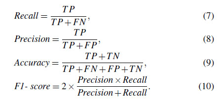
In defect detection, the choice of evaluation metrics is critical for real-world manufacturing
decisions. Although accuracy measures overall correctness across all classes, it
can be misleading in imbalanced scenarios since a model that predicts only the majority
class may still achieve high accuracy but miss most defects. Recall, on the other
hand, is vital because it measures how many actual defects are correctly identified;
missing a single defect can have severe cost, safety, or reliability implications.
Precision complements recall by indicating how many predicted defects are genuinely
defective, thus minimizing false positives that could disrupt manufacturing or re-inspection
efforts. Finally, the F1-score harmonizes recall and precision, balancing the need
to catch every defect with the need to avoid excessive false alarms. Focusing on these
metrics---especially recall and F1-score---ensures the model robustly identifies defects
without overwhelming production lines with unnecessary rechecks, ultimately supporting
a more reliable and efficient defect detection process. The mathematical definitions
of these metrics are as follows:
Table 2. The confusion matrix.
True Class
|
Predicted Class
|
Minority
|
Majority
|
Minority
|
True Positive
(TP)
|
False Negative (FN)
|
Majority
|
False Positive
(FP)
|
True Negative
(TN)
|
3. XCNet Implementation
The overall framework of XCNet is illustrated in Fig. 1. The model processes sensor input with a resolution of $H\times W$ and $C$ channels,
where $H=W=224$ and $C=3$. The input image passes through a feature extraction network
comprising five convolutional blocks, each consisting of a 2D convolutional layer
with a $3 \times 3$ filter, a dilation rate of $1 \times 1$, and zero padding to preserve
spatial dimensions. Each convolutional layer is followed by a ReLU [26] activation function and a MaxPooling2D layer with a $2 \times 2$ filter size, which
reduces the spatial resolution of the feature map by half along both the height and
width axes while doubling the number of channels. After feature extraction, the output
feature map has dimensions $\frac{H}{32}\times \frac{W}{32}\times 512$.
A GlobalAveragePooling2D (GAP) layer is then applied to aggregate spatial information
into a single value per channel, resulting in a 512-dimensional feature vector. This
layer enables the network to focus on the presence of features rather than their spatial
location, reduces computational cost, and mitigates overfitting compared to flattening
layers. The GAP output is passed to a Multi-Layer Perceptron block comprising three
fully connected layers with output sizes of 256, 128, and 10, respectively. Each layer
is followed by a ReLU activation and a Dropout layer with a rate of 20% to regularize
the model by reducing overfitting. Finally, the MLP block output is passed through
a classifier layer, a fully connected layer with an output size of 2 (one for each
class), which employs a softmax activation function to generate a probability distribution.
The class with the highest probability is selected as the predicted output for the
given image.
4. Result Analysis on XCNet
In this section, we first investigate the impact of each component of the XCNet model
on classification performance, followed by an analysis of how the quality of training
data influences model effectiveness.
4.1 Ablation Study
The ablation study presented in Table 3 investigates the impact of varying the number of convolutional blocks and filter
configurations on classification performance under different levels of class imbalance.
Additionally, it provides a comprehensive analysis of computational efficiency, including
model complexity (parameter count and GFLOPs) and inference speed, critical factors
for real-time defect detection in industrial settings. The dataset consists of two
training ratios, 1:10 and 1:50, representing different levels of minority class underrepresentation.
Four architectures were explored with convolutional blocks configured as [32, 64,
128], [32, 64, 128, 256], [16, 32, 64, 128, 256], and [32, 64, 128, 256, 512]. These
configurations progressively increase network depth and filter sizes, enhancing feature
extraction and enabling finer defect detection. Larger filters improve receptive fields,
capturing structural variations in sensor board defects while maintaining computational
efficiency.
For the 1:10 ratio, deeper architectures, such as AN3 ([16, 32, 64, 128, 256]) and
A.N. 4 ([32, 64, 128, 256, 512]), significantly outperformed shallower configuration.
These models achieved high accuracy (99.09% and 99.55%, respectively) and precision
(100%), while also improving recall for the minority class (90.90% and 95.45%). The
F1-scores of these configurations (95.23% and 95.45%) highlight their ability to balance
sensitivity and precision effectively. Conversely, shallower architectures, like A.N.
1 ([32, 64, 128]), show significant drop in recall, achieving only 40.90% and F1-score
of 58.05%, despite maintaining high overall accuracy (94.09%).
For the 1:50 ratio scenario, the performance gap between shallow and deep architectures
became even more visible due to the severe class imbalance. A.N. 5 ([32, 64, 128])
struggled, with a minority class recall of 21.05% and an F1-score of 33.33%, demonstrating
its limitations in handling extreme imbalance. In contrast, the A.N. 8 ([32, 64, 128,
256, 512]) architecture achieved the better performance, with an accuracy of 98.61%,
precision (100%), and an F1-score of 91.42%. This configuration showed substantial
improvements in recall (84.21%), indicating its effectiveness in capturing minority
class instances even in highly imbalanced scenarios.
Computational efficiency and scalability. Shallower models (A.N.~1, A.N.~5) have fewer
parameters (0.2~M) and lower FLOPs (1.18~G) but struggle to capture minority-class
instances effectively. Deeper architectures generally require more resources but substantially
improve recall. For example, A.N.~3 retains the same 1.0~M parameters like A.N.~2
but reduces FLOPs (0.90~G vs.~1.75~G) and inference time (3.75~ms vs.~4.65~ms), while
achieving better performance due to enhanced feature extraction. Building on this,
A.N.~4, which employs larger convolutional filters, has 4.0~M parameters and 2.31~G
FLOPs, but maintains an inference time of 5.63~ms, making it a viable option for real-time
applications while delivering the highest recall and F1-score.
These findings confirm that increasing the network depth and filter size improves
performance in heavily imbalanced scenarios but also offer competitive inference speeds,
making deeper architectures like A.N. 4 and A.N. 8 suitable for real-world manufacturing
environments where real-time defect detection is critical.
Table 3. Ablation study on number of convolution blocks and filter configuration.
Here, ``AN'' denotes the analysis number, ``Param (M)'' represents the model parameters
in millions, and ``Inf. (ms)'' indicates the inference speed in milliseconds. ``Acc.''
stands for accuracy, while ``Pre.'' refers to precision.
AN
|
Data
(Defect, Good)
|
Convolution Blocks
& Filters
|
Complexity
|
Evaluation Metrics (%)
|
Confusion Matrix
|
Param
(M)
|
FLOP
(G)
|
Inf. (ms)
|
Acc.
|
Pre.
|
Recall
|
F1-
Score
|
[TP, FN, FP, TN]
|
1
|
Train:
(80, 800)
Ratio: 1:10
Test: (22,19)
|
[32, 64, 128]
|
0.2
|
1.18
|
4.03
|
94.09
|
100
|
40.90
|
58.05
|
[9, 13, 0, 198]
|
2
|
[32, 64, 128, 256]
|
1.0
|
1.75
|
4.65
|
95.90
|
100
|
59.09
|
74.28
|
[13, 9, 0, 198]
|
3
|
[16, 32, 64, 128, 256]
|
1.0
|
0.59
|
3.75
|
99.09
|
100
|
90.90
|
95.23
|
[20, 2, 0, 198]
|
4
|
[32, 64, 128, 256, 512]
|
4.0
|
2.31
|
5.63
|
99.55
|
100
|
95.45
|
97.67
|
[21, 1, 0, 198]
|
5
|
Train:
(16, 800) Ratio: 1:50
Test: (19,19)
|
[32, 64, 128]
|
0.2
|
1.18
|
6.71
|
92.62
|
80
|
21.05
|
33.33
|
[4, 15, 1, 197]
|
6
|
[32, 64, 128, 256]
|
1.0
|
1.75
|
4.58
|
94.93
|
90
|
47.36
|
62.06
|
[9, 10, 1, 197]
|
7
|
[16, 32, 64, 128, 256]
|
1.0
|
0.59
|
3.82
|
97.69
|
93
|
78.95
|
85.70
|
[15, 4, 1, 197]
|
8
|
[32, 64, 128, 256, 512]
|
4.0
|
2.31
|
5.49
|
98.61
|
100
|
84.21
|
91.42
|
[16, 3, 0, 198]
|
4.2 Analysis of Data Distribution on Model Performance
This section provides an in-depth analysis of how variations in the composition of
training data affect the performance metrics of the model in two cases, Case I and
Case II. In Case I, the model is trained with the original data distribution, while
in Case II, the minority class sample is augmented. Details of the dataset are discussed
in Subsection 4.1.
Fig. 3 shows four graphs, each illustrates the performance metrics (accuracy, precision,
recall and F1-Score) for both cases, plotted against the fraction of the total good-class
training images. The x-axis represents the fraction of 800 good-class images used
for training, while the number of minority-class images is fixed at 28 for Case I
and 80 for Case II. The testing dataset remains constant in both cases. This comparative
evaluation demonstrates the significant impact of data distribution, particularly
the size of the minority class, on model performance.
Fig. 3(a) illustrates the accuracy metrics used to analyze the impact of data distribution
on model performance. In both cases, the model's accuracy progressively improves as
the fraction of good-class training data increases. However, Case II starts with a
higher initial accuracy (approximately 80%) and reaches near-perfect accuracy (100%)
much faster than Case I. This rapid improvement can be attributed to the larger minority-class
size in Case II, which mitigates class imbalance and allows the model to effectively
learn the dominant class, even with limited good-class training data. In contrast,
the improvement in Case I is slower, likely due to its smaller minority class, which
creates a greater imbalance and requires additional good-class training data to achieve
comparable accuracy. Overall, Case II demonstrates a clear advantage in accuracy across
all training levels, highlighting the critical role of managing class distributions
to optimize model performance.
As shown in Fig. 3(b), precision follows a similar trend, with Case II achieving near 100% precision early,
whereas Case I exhibits a more gradual increase. The superior performance of Case
II can be attributed to its larger minority-class size, which helps reduce overall
class imbalance. This improved balance enables the model to effectively minimize false
positives, even with limited good-class training data. In contrast, Case I, with its
smaller minority class, struggles to achieve comparable precision under similar conditions.
Fig. 3(c) highlights model performance in terms of recall stability and sensitivity under different
data distributions. Unlike accuracy and precision, which show stable and gradual improvement
as training data increases, recall behaves differently. In Case I, recall fluctuates
at lower training fractions, with noticeable dips indicating inconsistent sensitivity
in detecting the minority class. This instability likely arises from the smaller minority-class
size in the training dataset. In contrast, recall in Case II remains consistently
high across all training fractions, demonstrating the model's robustness in detecting
the minority class. The larger minority class in Case II mitigates class imbalance,
ensuring that the good class receives adequate representation during training.
Fig. 3(d) illustrates the F1-score, which combines precision and recall into a single metric
to provide a holistic measure of the model's classification performance. Case II consistently
outperforms Case I, with a rapid increase in F1-score that stabilizes near 100%, even
at lower fractions of good-class training data. This superior performance can be attributed
to Case II's larger minority-class size, which enhances the model's ability to distinguish
between classes and reduces the trade-off between precision and recall. In contrast,
Case I shows a slower, more gradual improvement in F1-score, remaining consistently
lower across all training levels. This slower progression reflects challenges in balancing
precision and recall caused by the smaller minority class, which intensifies class
imbalance and limits the model's ability to optimize performance with less training
data.
The key observations and implications are as follows: One significant finding is the
impact of minority-class size on model performance. Case II, with a larger minority-class
size, consistently outperforms Case I across all metrics, demonstrating that a more
balanced class distribution improves the model's learning and generalization. Another
important insight is the sufficiency of training data. Case II achieves near-optimal
performance with fewer training images, highlighting the efficiency of balanced datasets
in achieving high accuracy and other key metrics with reduced data. Both cases show
performance improvements as training data increases. However, Case II excels in accuracy,
precision, recall, and F1-score, even with smaller training fractions. This stability
underscores the importance of balanced class distributions for reliable and consistent
model performance.
Fig. 3. Data quality study. The plots show the effect of varying the proportion of
good quality training data on (a) Accuracy, (b) Precision, (c) Recall, and (d) F1-Score
for two cases: Case I (original data) and Case II (augmentation data).
4.3 Result Analysis
Table 4 compares XCNet with other state-of-the-art (SOTA) models, including VGG16 [27], ResNet34 [28], ResNet50 [28], ViT-Tiny [29], and ViT-Base [29], all pretrained on ImageNet1k. While these models perform well on large-scale datasets,
they struggle to adapt to the small, domain-specific defect dataset, particularly
in cases of severe class imbalance. ViT-Base, for instance, with 86.90 million parameters
and 17.58 GFLOPs, fails to surpass XCNet's performance, likely due to the limited
training data ($<1000$ images) and the domain shift from natural images to industrial
defect images.
In contrast, XCNet delivers higher recall and F1-scores under both 1:10 and 1:50 imbalances,
attaining 99.45% and 98.62% accuracy, respectively, while also maintaining perfect
precision (100%). From a complexity standpoint, XCNet requires substantially fewer
parameters (4.0~M) and GFLOPs (2.31~G) than the larger SOTA models---VGG16 with 138.36~M
parameters and 15.47~GFLOPs or ViT-Base with 86.90~M parameters and 17.58~GFLOPs.
This efficient combination of strong performance and moderate computational requirements
underscores XCNet's suitability for real-world manufacturing scenarios, where data
are scarce and real-time defect detection is critical.
Table 4. Result Comparison with other state-of-the-art models. Here, Inference (ms)
refers to model inference time in mili-seconds. Best result is shown in bold.
Data
(Defect, Good)
|
Model
|
Complexity
|
Evaluation Metrics (%)
|
Confusion
|
Param
(M)
|
FLOP
(G)
|
Inference (ms)
|
Accuracy
|
Precision
|
Recall
|
F1-score
|
[TP, FN, FP, TN]
|
Train:
(80,800)
Ratio: 1:10
Test:
(22:198)
|
VGG16 [27]
|
138.36
|
15.47
|
11.60
|
98.18
|
95
|
86.36
|
90.47
|
[19, 3, 1, 197]
|
ResNet34 [28]
|
22.10
|
3.67
|
8.16
|
98.64
|
95.23
|
90.90
|
93.01
|
[20, 2, 1, 197]
|
ResNet50 [28]
|
25.90
|
4.11
|
9.34
|
99.45
|
100
|
95.45
|
97.67
|
[21, 1, 0, 198]
|
ViT-Tiny [29]
|
5.80
|
1.26
|
5.45
|
99.09
|
100
|
90.90
|
95.23
|
[20, 2, 0, 198]
|
ViT-Base [29]
|
86.90
|
17.58
|
12.02
|
99.45
|
100
|
95.45
|
97.67
|
[21, 1, 0, 198]
|
XCNet
|
4.00
|
2.31
|
5.63
|
99.45
|
100
|
95.45
|
97.67
|
[21, 1, 0, 198]
|
Train: (16,800)
Ratio: 1:50
Test: (19:198)
|
VGG16 [27]
|
138.36
|
15.47
|
11.23
|
94.47
|
70.59
|
63.16
|
66.67
|
[12, 7, 5, 193]
|
ResNet34 [28]
|
22.10
|
3.67
|
8.35
|
95.39
|
73.68
|
73.68
|
73.68
|
[14, 5, 5, 193]
|
ResNet50[28]
|
25.90
|
4.11
|
9.29
|
96.31
|
82.35
|
73.68
|
77.77
|
[14, 5, 3, 195]
|
ViT-Tiny [29]
|
5.80
|
1.26
|
5.37
|
95.85
|
77.78
|
73.68
|
75.67
|
[14, 5, 4, 194]
|
ViT-Base [29]
|
86.90
|
17.58
|
11.72
|
98.16
|
100
|
78.94
|
88.23
|
[15, 4, 0, 198]
|
XCNet
|
4.00
|
2.31
|
5.49
|
98.62
|
100
|
84.21
|
91.43
|
[16, 3, 0, 198]
|
4.4 Analysis on Overfitting to Synthetic Patterns
Figs. 4 and 5 analyze the potential risk of overfitting, specifically whether the model learns
artificial patterns from data augmentation instead of genuine defect features. To
investigate this, we applied augmentation only to the minority class in both the training
and test datasets. Each augmented set includes both original and modified images,
ensuring that synthetic images do not dominate the evaluation.
In Fig. 4, the training loss (showing results from the original training dataset; other graphs
with similar trends are omitted for clarity) remains steady and stable, while test
losses across various augmentations (e.g., flipped images) show no abrupt spikes---indicating
that the model learns robust features rather than memorizing synthetic patterns. Fig.~5
further underscores this robustness by showing steady improvements in recall and F1-scores
for each augmented scenario. The fact that performance consistently increases as more
augmentations are introduced suggests that XCNet acquires generalizable defect features
rather than relying on artificially introduced cues. This combined findings strongly
support the effectiveness of our augmentation strategy in helping XCNet learn meaningful
defect characteristics without overfitting to synthetic patterns.
Fig. 4. Training and test loss under various augmentation scenarios.
Fig. 5. Recall and F1-Scores comparisons across different augmentation scenarios.
4.5 Adaptability to Other Semiconductor Products
Although our work focuses on sensor board defect detection, XCNet can easily be adapted
to other semiconductor components and industrial products. Numerous studies confirm
the versatility of CNN-based architectures for various defect detection tasks, from
wafer map analysis [30] to surface flaw identification [31,32]. Transfer learning has further demonstrated CNN adaptability to different data distributions
[33,34]. Building on these findings, XCNet's emphasis on efficient feature extraction and
robust classification requires only minimal adjustments---such as domain-specific
data augmentation or slight architectural tweaks---to detect defects across diverse
industrial contexts. This adaptability highlights XCNet's potential to make a broader
impact on semiconductor inspection and defect detection in a wide range of manufacturing
scenarios.
V. CONCLUSION
In this work, we introduced XCNet, a convolutional neural network-based solution for
automated defect detection in sensor boards. XCNet addresses the limitations of traditional
manual inspection methods by significantly improving inspection accuracy and efficiency
while minimizing human intervention, making it a robust tool for modern manufacturing
environments.
We conducted a comprehensive ablation study to evaluate the impact of XCNet's architectural
components on model performance. By experimenting with different numbers of convolutional
blocks and filter configurations, we demonstrated that deeper architectures consistently
outperformed shallower ones, particularly in handling class imbalance. These configurations
achieved high accuracy while showing substantial improvements in minority class recall
and F1-scores.
Our analysis further highlighted the critical role of data quality and class balance
in determining model performance. The study on data augmentation for the minority
class showed significant advantages, achieving near-perfect accuracy and precision
with fewer training samples. These findings underscore the importance of both architectural
design and data preprocessing in improving model performance for imbalanced classification
tasks. By automating defect detection, XCNet reduces costs, enhances efficiency, and
ensures product reliability. This work contributes to the advancement of intelligent
manufacturing systems, providing valuable insights for addressing class imbalance
and optimizing deep learning models for quality control.
References
J. Serey, M. Alfaro, G. Fuertes, M. Varhas, C. Durán, R.
Ternero, R. Rivera, and J. Sabattin, ``Pattern recognition and deep learning
technologies, enablers of Industry 4.0, and their role in engineering research,''
Symmetry, vol. 15, no. 2, 535, 2023.

J. Wang, Y. Ma, L. Zhang, R. X. Gao, and D. Wu, ``Deep learning for smart manufacturing:
Methods and applications,'' Journal of Manufacturing Systems, vol. 48, pp. 144-156,
2018.

S. Sundaram and A. Zeid, ``Artificial intelligence-based smart quality inspection
for manufacturing,'' Micromachining, vol. 14, no. 2, 570, 2023.

E. Baran and T. K. Polat, ``Classification of Industry 4.0 for total quality management:
A review,'' Sustainability, vol. 14, no. 6, 3329, 2022.

T.P. Nguyen, S. Choi, S.J. Park, and J. Yoon, ``Inspecting method for defective casting
products with convolutional neural network (CNN),'' International Journal of Precision
Engineering and Manufacturing-Green Technology, vol. 8, pp. 583-594, 2021.

F. Pernkopf and P. O'Leary, ``Visual inspection of machined metallic high-precision
surfaces,'' EURASIP Journal on Advances in Signal Processing, vol. 2002, pp. 1-12,
2002.

X. Jiang, P. Scott, and D. Whitehouse, ``Wavelets and their applications for surface
metrology,'' CIRP Annals, vol. 57, no. 1, pp. 555-558, 2008.

D. H. Harris, ``The nature of industrial inspection,'' Human Factors, vol. 11, no.
2, pp. 139-148, 1969.

J. E. See, ``Visual inspection reliability for precision manufactured parts,'' Human
Factors, vol. 57, no. 8, pp. 1427-1442, 2015.

D. Weimer, B. Scholz-Reiter, and M. Shpitalni, ``Design of deep convolutional neural
network architectures for automated feature extraction in industrial inspection,''
CIRP Annals, vol. 65, no. 1, pp. 417-420, 2016.

F. Riaz, K. Kamal, T. Zafar, and R. Qayyum, ``An inspection approach for casting defects
detection using image segmentation,'' Proc. of 2017 International Conference on Mechanical,
System and Control Engineering (ICMSC), pp. 101-105, 2017.

M. Ferguson, R. Ak, Y.-T. T. Lee, and K. H. Law, ``Automatic localization of casting
defects with convolutional neural networks,'' Proc. of 2017 IEEE International Conference
on Big Data (Big Data), pp. 1726-1735, December 2017.

M. I. Jordan and T. M. Mitchell, ``Machine learning: Trends, perspectives, and prospects,''
Science, vol. 349, no. 6245, pp. 255-260, 2015.

H. Xie and Z Wu, ``A robust fabric defect detection method based on improved RefineDet,''
Sensors, vol. 15, no. 15, 2020.

P. Murray, E. Yakushina, S. Marshall, and W. Lon, ``Automated microstructural analysis
of titanium alloys using digital image processing,'' IOP Conference Series: Materials
Science and Engineering, vol. 179, 012011, 2017.

M. M. Islam, A. A. Mintoo, and A. S. M. Saimon, ``Enhancing textile quality control
with IoT sensors: A case study of automated defect detection, Global Mainstream Journal,
vol. 1, no. 1, pp. 19-30, 2024.

J. Breitenbach, I. Eckert, V. Mahal, H. Baumgartl, and R. Buettner, ``Automated defect
detection of screws in the manufacturing industry using convolutional neural networks,''
Proc. of the 55th Hawaii International Conference on System Sciences, 2022.

L. Song, X. Li, Y. Yang, X. Zhu, Q. Guo, and H. Yang, ``Detection of micro-defects
on metal screw surfaces based on deep convolutional neural networks,'' Sensors, vol.
18, no. 11, 2018.

Z. Liu, B. Tian, X. Li, C. Li, and Y. Dong, ``Saliency-based fabric defect detection
network with feature pyramid learning and refinement,'' Proc. of Fourteenth International
Conference on Graphics and Image Processing (ICGIP 2022), vol. 12705, 127050N, 2023.

S. Zhou, Y. Chen, D. Zhang, J. Xie, and Y. Zhou, ``Classification of surface defects
on steel sheet using convolutional neural networks,'' Materiali in Tehnologije/Materials
and Technology, vol. 51, no. 1, pp. 123-131, 2017.

A. S˛eker, K. A. Peker, A. G. Yüksek, and E. Delibas, ``Fabric defect detection using
deep learning,'' Proc. of 2016 24th Signal Processing and Communication Application
Conference (SIU), IEEE, pp. 1437-1440, 2016.

S.-H. Huang and Y.-C Pan, ``Automated visual inspection in the semiconductor industry:
A survey,'' Computers in Industry, vol. 66, pp. 1-10, 2015.

Y. Qiao and L. Xing, ``Automatic classification method for Oracle images based on
deep learning,'' IEIE Transactions on Smart Processing and Computing, vol. 12, no.
2, pp. 87-96, April 2023.

S. P. Yadav, ``Vision-based detection, tracking, and classification of vehicles,''
IEIE Transactions on Smart Processing and Computing, vol. 9, no. 6, pp. 427-434, December
2020.

M. N. Nguyen and T. Nguyen, ``Deep learning approaches to human gait pattern classification
based on MEMS sensors,'' IEIE Transactions on Smart Processing and Computing, vol.
9, no. 4, pp. 184-292, August 2020.

J. He, L. Li, J. Xu, and C. Zheng, ``ReLU deep neural networks and linear finite elements,''
Journal of Computational Mathematics, vol. 38, no. 3, pp. 502-527, July 2018.

S. Karen and Z. Andrew, ``Very deep convolutional networks roe large-scale image recognition,''
arXiv preprint arXiv:1409.1556, 2014.

K. He, X. Zhang, S Ren, and J. Sun, ``Deep residual learning for image recognition,''
Proc. of the IEEE Conference on Computer Vision and Pattern Recognition, pp. 770-778,
2016.

A. Dosovitskiy, ``An image is worth 16x16 words: Transformers for image recognition
at scale,'' arXiv preprint arXiv:2010.11929, 2020.

Y. F. Yang and M. Sun, ``Semiconductor defect detection by hybrid classical-quantum
deep learning,'' Proc. of the IEEE/CVF Conference on Computer Vision and Pattern Recognition,
pp. 2323-2332, 2022.

D. Ujalambkar, C. Kulkarni, V. Navale, and N. P. Sable, ``Industrial product surface
defect detection using CNN: A deep learning approach,'' Panamerican Mathematical Journal,
vol. 34, no. 3, 2024

S. Arikan, K. Varanasi, and D. Stricker, ``Surface defect classification in real-time
using convolutional neural networks,'' arXiv preprint arXiv:1904.04671, 2019.

B. Devika and N. George, ``Convolutional neural network for semiconductor wafer defect
detection,'' Proc. of 2019 10th International Conference on Computing, Communication
and Networking Technologies (ICCCNT), pp. 1-6, 2019.

J. Yang, S. Li, Z. Wang, H. Dong, J. Wang, and S. Tang, ``Using deep learning to detect
defects in manufacturing: A comprehensive survey and current challenges,'' Materials,
vol. 13, no. 24, 5755, 2020.

Sachin Ranjan received his diploma from Tribhuvan University, Nepal, in 2015 and
his B.E. degree from Uttarakhand Technical University, India, in 2019. He is currently
pursuing an M.S. degree in electronics engineering at Incheon National University
(INU), South Korea, where he is working as a Research Assistant at the Machine Intelligence
and Data Science (MINDS) Lab. His research interests include image processing, machine
learning, computer vision, robotics, 6G mobile communication systems, and the Internet
of Things (IoT).
Hoon Kim received his B.S. degree in electrical engineering from Korea Advanced
Institute of Science and Technology (KAIST), Korea in 1998, and his M.S. and Ph.D.
degrees in engineering from Information and Communication University (ICU), Korea
in 1999 and 2004, respectively. He had been working with Samsung Advanced Institute
of Technology (SAIT) during 2004 to 2005, while serving as a Senior Engineer in Communications
and Networks Laboratory Division joining the project of design and performance analysis
of radio transmission technology for beyond 3G and 4G mobile communication systems.
He also had been working with Ministry of Information and Communications (MIC) from
2005 to 2007 as a deputy director in Broadband Communications Division in charge of
promotion policies on broadband communications industry such as WiMAX. He joined Stanford
University as a visiting scholar and a visiting professor during 2007 to 2008 and
2014 to 2015, respectively, and worked on developing radio resource management algorithms
and cross layer optimization schemes for 4/5G mobile communications systems. He is
currently a Professor of the Department of Electronics Engineering at Incheon National
University where he has been working with the same department since 2008. His research
interests include 6G mobile communication systems, internet of things, artificial
intelligence, and big data. He is a Member of KICS, IEIE, IEEE, and IEICE.